EARTH AS A TELESCOPE / INTERACTIVE ATLAS
IceCube Neutrino Detector
Catch a cosmic messenger beneath Antarctica
A visitor crosses the universe. Deep beneath Antarctica, a handful of flashes becomes a clue. Enter the ice, illuminate a teaching event, and ask how much a direction can tell you.
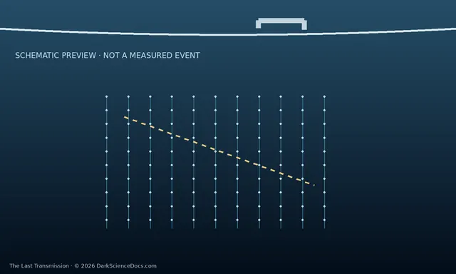
IceCube is a neutrino observatory at the South Pole. Sensors deep in Antarctic ice detect Cherenkov light emitted by charged particles produced when neutrinos interact in or near the detector. The pattern and timing of these flashes help scientists estimate a particle’s direction and energy. This interactive 3D Atlas uses synthetic events to explain the method; it does not display recorded IceCube observations.
01 / BENEATH THE WORLD
The telescope is the ice.
Load the expedition, then descend. Drag to orbit; pinch or use + and − to zoom. On phones, hold the arrows inside the view. The station exterior and snow are an illustrative reconstruction inspired by IceCube field photographs; building dimensions, equipment placement and string positions are approximate. Sensor markers are enlarged for visibility.
The 3D scene loads only on request. The timing exercise below also works if 3D is unavailable.
Event settings
Synthetic teaching eventDirections use this model’s local axes, not celestial coordinates. Light yield is an illustrative brightness setting, not calibrated energy.
Every event here is generated for learning. No replay is an IceCube observation.
A few modeled microseconds are stretched into an eight-second replay. Color marks relative arrival time. The model simplifies ice optics, sensor response and particle interactions; hits are not detector-calibrated charges. The gold arrow is the path and direction of a simulated muon, not a visible neutrino beam. Round colored markers are sensors receiving light; their colors encode arrival time, not the light’s actual color. Real data also contain background muons: a track alone does not establish a neutrino source.
02 / FOLLOW THE TIMING
Where might it have come from?
Can the sensor timing recover the direction we put into the simulation? Analyze the complete event, then reveal the known input. This plots where the particle came from—the opposite of the travel direction set above.
- Estimated incoming direction
- Analyze an event first
- Known simulation input
- Hidden until revealed
- Angular difference
- Reveal the input to compare
The fit uses synthetic sensor positions and first-arrival times. It is not IceCube’s reconstruction pipeline.
A smaller angular difference means a closer match within this exercise; it does not measure IceCube’s real pointing accuracy. Azimuth means angle around the model; elevation means angle above or below its horizontal plane. 0° and 360° are the same direction. These are not celestial sky coordinates. The pointlike cascade model contains no directional light structure, so this simple fit deliberately does not assign it a source direction. Real cascade analyses can infer directions using more information.
03 / THREE MESSENGERS
Which message gets through?
Give the source more obscuring material or a stronger magnetic deflection. Compare what reaches the observer in this schematic.
In this attenuation-only example, about 14% of gamma rays remain in the direct beam at τ = 2.
The gamma-ray fraction is e−τ for the chosen schematic energy and optical depth; no energy scale is specified. Magnetic fields bend charged particles. Neutrinos are uncharged and rarely interact, but are not guaranteed to pass through arbitrary matter at every energy. Equal animation speeds do not compare physical travel times.
FROM YOUR TRIAL TO THE PUBLISHED RECORD
One event is not a galaxy.
Your synthetic track illustrates how timing can constrain a direction. A real source association also needs backgrounds, uncertainty, exposure and many events. The NGC 1068 result is a statistical analysis of an obscured active galaxy, not a claim that the event you just generated came from it.
The public release contains analysis inputs and scripts. This Atlas does not download that dataset or reproduce the published source-significance calculation. Replaying this scene is not a replication of that research.
What this model keeps—and leaves out.
The original array’s count and broad depth range are retained, while positions are an approximate layout with a denser central group. The compact overview shortens the empty-ice gap and enlarges the surface model 8× for legibility; its depth-break mark signals this change of display scale. Detector, Inside and Surface views retain their modeled coordinates, and event calculations always use the original sensor positions. Exact surveyed string locations, detailed DeepCore placement, layered scattering and absorption, noise, detector efficiencies and full event reconstruction are omitted. Buildings, wind-shaped snow and ice textures, light waves and cutaway visibility are illustrative; the surface is not a surveyed Antarctic terrain map. This is the original 86-string configuration; the 2026 Upgrade added five strings and further instrumentation, which are not shown.
The timing exercise uses a fixed refractive index of 1.32, a secondary track moving approximately at vacuum light speed, and simplified earliest photon travel times. Its linear fit is a teaching approximation, not a likelihood analysis. A small error against known simulated truth does not measure real-detector accuracy. Increasing light yield changes a synthetic hit threshold, not the probability that an arbitrary cosmic neutrino will interact.
- IceCube: original detector configuration and detection principle
- IceCube: the 2026 Upgrade and its additional instrumentation
- IceCube: track reconstruction and directional uncertainty
- IceCube: tracks, cascades and source analysis
- IceCube: NGC 1068 and its obscured environment
- IceCube: how a muon track and time-colored sensor detections appear in a measured event display
- IceCube field photographs: laboratory exterior, cable reels and snow-covered work areas